论文链接:Classifier-Free Diffusion Guidance

上一篇文章我们学习了 Classifier Guidance,这种方法通过引入一个额外的分类器,使用梯度引导的方式成功地实现了条件生成。虽然 Classifier Guidance 可以直接复用训练好的 diffusion models,不过这种方法的问题是很明显的,首先需要额外训练一个分类器,而且这个分类器不仅仅分类一般的图像,还需要分类加噪后的图像,这会给方法带来比较大的额外开销;其次分类器训练完成后类别就固定下来了,如果希望生成新的类别就需要重新训练分类器。这篇文章学习的 Classifier-Free Guidance 则可以比较好地解决这些问题。

Classifier-Free Guidance

在 Classifier Guidance 中,从条件概率 \(p(\mathbf{x}_t|y)\) 出发,利用贝叶斯公式和 score function 推导出了以下公式,在下面的公式中,等号右侧的第一项已知,第二项则需要引入分类器进行计算。 \[ \nabla_{\mathbf{x}_t}\log p(\mathbf{x}_t|y)=\underbrace{\nabla_{\mathbf{x}_t}\log p(\mathbf{x}_t)}_{\textrm{unconditional}~\textrm{score}}+\underbrace{\nabla_{\mathbf{x}_t}\log p(y|\mathbf{x}_t)}_{\textrm{adversarial}~\textrm{gradient}} \] 并且在实际使用时,为了调节控制的强度,会引入一个额外的叫做 guidance scale 的参数 \(s\)。最终的结果是以 \(s\) 作为权重进行加权的结果,也就是: \[ \nabla_{\mathbf{x}_t}\log p(\mathbf{x}_t|y)=\nabla_{\mathbf{x}_t}\log p(\mathbf{x}_t)+s\nabla_{\mathbf{x}_t}\log p(y|\mathbf{x}_t) \] 现在我们不希望使用分类器来计算 \(\nabla_{\mathbf{x}_t}\log p(y|\mathbf{x}_t)\) 这一项,因此需要用另一种方式来表示这一项,把第一个公式中的这一项移到等号左侧: \[ \nabla_{\mathbf{x}_t}\log p(y|\mathbf{x}_t)=\nabla_{\mathbf{x}_t}\log p(\mathbf{x}_t|y)-\nabla_{\mathbf{x}_t}\log p(\mathbf{x}_t) \] 然后再代入第二个含有参数 \(s\) 的公式: \[ \begin{aligned} \nabla_{\mathbf{x}_t}\log p(\mathbf{x}_t|y)&=\nabla_{\mathbf{x}_t}\log p(\mathbf{x}_t)+s\nabla_{\mathbf{x}_t}\log p(y|\mathbf{x}_t)\\ &=\nabla_{\mathbf{x}_t}\log p(\mathbf{x}_t)+s\left(\nabla_{\mathbf{x}_t}\log p(\mathbf{x}_t|y)-\nabla_{\mathbf{x}_t}\log p(\mathbf{x}_t)\right)\\ &=\underbrace{(1-s)\nabla_{\mathbf{x}_t}\log p(\mathbf{x}_t)}_{\textrm{unconditional}~\textrm{score}}+\underbrace{s\nabla_{\mathbf{x}_t}\log p(\mathbf{x}_t|y)}_{\textrm{conditional}~\textrm{score}} \end{aligned} \] 到这一步就已经得到 classifier-free guidance 的形式了。在上边的式子里第一项对应于无条件生成的分数,第二项对应于有条件生成的分数,\(s\) 是一个用来控制条件重要性的参数,当 \(s=0\),模型就是原来的无条件生成模型;当 \(s=1\),模型完全依赖于条件;当 \(s>1\),模型不仅更加重视条件,而且向远离无条件生成的方向移动。一般来说参数的取值为 \(s=7.5\),之所以不在 0 到 1 之间取值是因为我们想生成的并不是介于「无条件生成」和「有条件生成」之间的一种似是而非的样本,而是非常明确符合条件的结果,因此这个参数的取值是比较大的。

上边的公式也可以写成另一种形式,如下所示。两项分别是无条件生成的分数以及从无条件生成指向有条件生成的方向,这样看就更清晰了:classifier-free guidance 就是从无条件生成的基础上向某个条件的方向移动。 \[ \nabla_{\mathbf{x}_t}\log p(\mathbf{x}_t|y)=\underbrace{\nabla_{\mathbf{x}_t}\log p(\mathbf{x}_t)}_{\textrm{unconditional}~\textrm{score}}+\underbrace{s(\nabla_{\mathbf{x}_t}\log p(\mathbf{x}_t|y)-\nabla_{\mathbf{x}_t}\log p(\mathbf{x}_t))}_{\textrm{unconditional}~\textrm{to}~\textrm{conditional}} \] 不过这个方法也有一些不容易理解的地方,观察一下公式可以发现 \(\nabla_{\mathbf{x}_t}\log p(\mathbf{x}_t|y)\) 这一项同时出现在了等式的左侧和右侧,那么如果想学习 \(\nabla_{\mathbf{x}_t}\log p(\mathbf{x}_t|y)\),直接对这一项进行学习就可以了,为什么还需要拆分成无条件生成和有条件生成两部分呢?根据我个人的理解,从上边的式子可以看出无条件生成是有条件生成的基础,生成的质量和多样性是由无条件生成的分数保证的,如果只有有条件生成而没有无条件生成,那么生成效果可能不佳。

训练与采样过程

从上一节我们已经知道了可以通过分别对无条件生成和有条件生成进行学习,得到无需分类器的有条件生成模型。那么需要学习的有两种模型,具体来说就是一个只输入带噪声图像的模型 \(\epsilon_\theta(\mathbf{x})\) 和一个同时输入噪声图和条件的模型 \(\epsilon_\theta(\mathbf{x},\mathbf{c})\)。不过原始论文的作者并没有这样做,因为使用两个模型的参数量比较大,并且实现比较复杂。要实现无条件生成,不一定要去掉额外的条件输入,直接把条件输入替换成某个固定的空值 \(\varnothing\) (例如 0)也是可以的。这样,有条件和无条件就被统一成了同一个模型 \(\epsilon_\theta(\mathbf{x},\mathbf{c})\),当 \(\mathbf{c}=\varnothing\) 就是无条件的情况。

为了联合训练有条件和无条件的情况,在训练时需要以一定的概率 \(p_\mathrm{uncond}\) 将条件输入替换为 \(\varnothing\)。其他的部分和一般的 diffusion model 的训练过程区别不大,论文中也给出了训练的算法,可以看到除了多了条件作为输入以及采样无条件生成的输入之外,没有其他的变化:

Classifier-Free Guidance 的训练流程

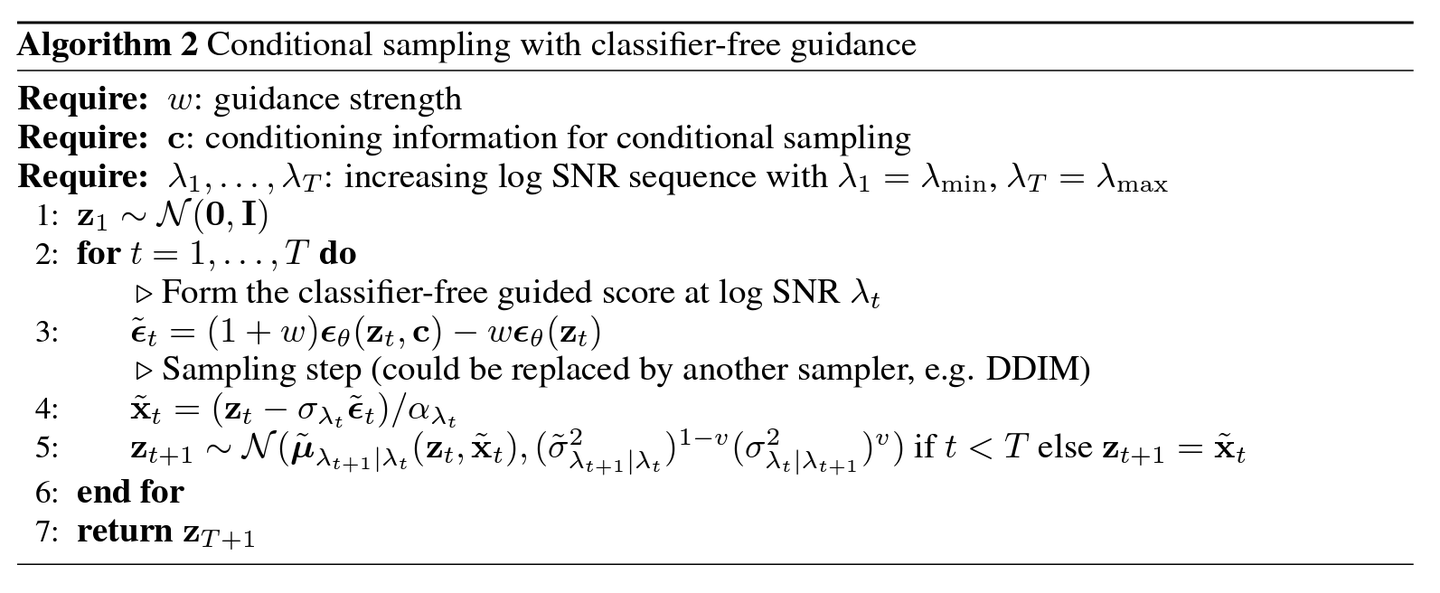
文中也给出了采样算法的流程,可以看到预测噪声由无条件和有条件两部分加权得到:

Classifier-Free Guidance 的采样流程

条件注入的方式

根据我们前文中的讨论,只需要给噪声预测模型加入一个条件参数,即可实现有条件去噪和无条件去噪。我们知道去噪模型通常使用的都是 UNet,将条件注入 UNet 有几种比较常见的方式,即交叉注意力、通道注意力以及自适应归一化等。

Cross Attention

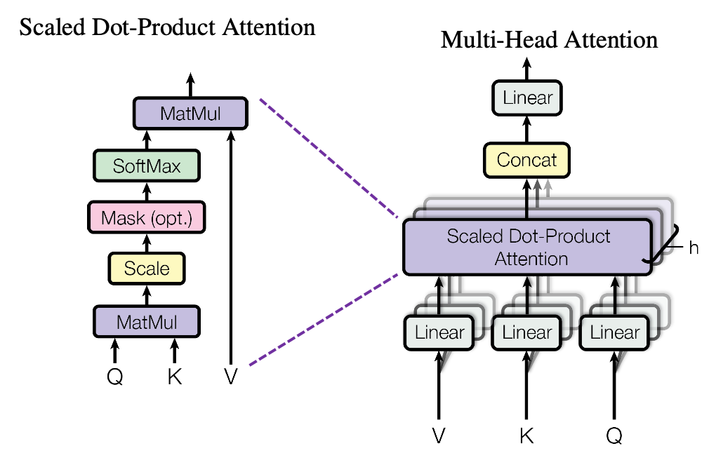
交叉注意力是比较常用的一种条件注入方式,例如很多文生图模型的文本就是用这种方式注入的。在注入时是以 \(\mathbf{x}\) 为 query、以 \(\mathbf{c}\) 为 key 和 value。可以以下面这张图中的结构做为参考看一下 diffusers 的代码。

Scaled Dot-Product Attention

diffusers 对 UNet 中使用的 attention 进行了多层封装,具体的层次结构如下所示:

1
2
3
4
5
6
7
8
9
10
11
diffusers.models.unets.unet_2d_condition.UNet2DConditionModel
+ 以下采样为例,这个类的 down_blocks 是一个 ModuleList,包含的部分模块为:
+ diffusers.models.unets.unet_2d_blocks.CrossAttnDownBlock2D
+ 该类的 attentions 属性也是一个 ModuleList,包含的模块为:
+ diffusers.models.transformers.transformer_2d.Transformer2DModel
+ 该类的 transformer_blocks 也是一个 ModuleList,包含的模块为:
+ diffusers.models.attention.BasicTransformerBlock
+ 该类的 attn1 和 attn2 是 attention 真正的实现,类型为:
+ diffusers.models.attention_processor.Attention
+ 该类内部还使用了一个 processor 来控制 attention 的类型,类型为:
+ diffusers.models.attention_processor.AttnProcessor2_0

在上述层次关系中,我们只需要关心最后两层,也就是 attention 的具体实现。我们把其中核心的代码拿出来看:

1
2
3
4
5
6
7
8
9
10
11
12
13
14
15
16
17
18
class Attention(nn.Module):
...
def forward(
self,
hidden_states: torch.Tensor,
encoder_hidden_states: Optional[torch.Tensor] = None,
attention_mask: Optional[torch.Tensor] = None,
**cross_attention_kwargs,
) -> torch.Tensor:
... # 一些预处理,此处省略

return self.processor(
self,
hidden_states,
encoder_hidden_states=encoder_hidden_states,
attention_mask=attention_mask,
**cross_attention_kwargs,
)

可以看到直接调用了 processor,那么我们再看这个类是怎么实现的,具体的解释可以直接看注释:

1
2
3
4
5
6
7
8
9
10
11
12
13
14
15
16
17
18
19
20
21
22
23
24
25
26
27
28
29
30
31
32
33
34
35
36
37
38
39
40
41
42
43
class AttnProcessor2_0: # 这个类实现了 scaled dot-product attention
...

def __call__(
self,
attn: Attention,
hidden_states: torch.Tensor, # 对应带噪声的图像,也就是 x
encoder_hidden_states: Optional[torch.Tensor] = None, # 对应条件,也就是 c
attention_mask: Optional[torch.Tensor] = None, # 此处忽略相关内容
temb: Optional[torch.Tensor] = None, # 此处忽略相关内容
*args,
**kwargs,
) -> torch.Tensor:
input_ndim = hidden_states.ndim
if input_ndim == 4: # 在做 attention 的时候需要把 spatial 维度压缩到同一维
batch_size, channel, height, width = hidden_states.shape
hidden_states = hidden_states.view(batch_size, channel, height * width).transpose(1, 2)
batch_size, sequence_length, _ = hidden_states.shape if encoder_hidden_states is None else encoder_hidden_states.shape
# 这里进行了 query 的编码,query 从 x 得到
query = attn.to_q(hidden_states)
# 如果没有条件,cross attention 就变成 self attention
if encoder_hidden_states is None:
encoder_hidden_states = hidden_states
# key 和 value 编码,从 c 得到
key = attn.to_k(encoder_hidden_states)
value = attn.to_v(encoder_hidden_states)
# multi-head attention 相关准备
inner_dim = key.shape[-1]
head_dim = inner_dim // attn.heads
query = query.view(batch_size, -1, attn.heads, head_dim).transpose(1, 2)
key = key.view(batch_size, -1, attn.heads, head_dim).transpose(1, 2)
value = value.view(batch_size, -1, attn.heads, head_dim).transpose(1, 2)
# 进行点积注意力
hidden_states = F.scaled_dot_product_attention(query, key, value, attn_mask=attention_mask, dropout_p=0.0, is_causal=False)
hidden_states = hidden_states.transpose(1, 2).reshape(batch_size, -1, attn.heads * head_dim)
# 后边的就都不重要了,是一些后处理,例如 linear projection、dropout
hidden_states = hidden_states.to(query.dtype)
hidden_states = attn.to_out[0](hidden_states)
hidden_states = attn.to_out[1](hidden_states)
if input_ndim == 4:
hidden_states = hidden_states.transpose(-1, -2).reshape(batch_size, channel, height, width)
hidden_states = hidden_states / attn.rescale_output_factor
return hidden_states

Channel-wise Attention

相比于交叉注意力,通道注意力相对比较简单。虽然叫注意力,但其实就是做完 projection 直接加到 time embedding 上,具体的代码可以参考 diffusers.models.embeddings.TimestepEmbedding

1
2
3
4
5
6
7
8
9
10
11
12
class TimestepEmbedding(nn.Module):
...
def forward(self, sample, condition=None):
if condition is not None: # 条件在这里注入
sample = sample + self.cond_proj(condition)
sample = self.linear_1(sample)
if self.act is not None:
sample = self.act(sample)
sample = self.linear_2(sample)
if self.post_act is not None:
sample = self.post_act(sample)
return sample

上述代码中的 cond_proj 的定义如下,可以看到就是一个 linear 层:

1
self.cond_proj = nn.Linear(cond_proj_dim, in_channels, bias=False)

这种注入方式一般用于比较简单的条件的注入,例如类别条件等。

Adaptive Normalization

自适应归一化有几种,比如自适应层归一化、自适应组归一化以及一些变体。这里以最简单的情况为例,在 diffusers 中的实现位于 diffusers.models.normalization.AdaLayerNorm,可以看到是利用 timestepx 进行了一个 affine 操作:

1
2
3
4
5
6
7
8
9
10
11
12
13
14
class AdaLayerNorm(nn.Module):

def __init__(self, embedding_dim: int, num_embeddings: int):
super().__init__()
self.emb = nn.Embedding(num_embeddings, embedding_dim)
self.silu = nn.SiLU()
self.linear = nn.Linear(embedding_dim, embedding_dim * 2)
self.norm = nn.LayerNorm(embedding_dim, elementwise_affine=False)

def forward(self, x: torch.Tensor, timestep: torch.Tensor) -> torch.Tensor:
emb = self.linear(self.silu(self.emb(timestep)))
scale, shift = torch.chunk(emb, 2)
x = self.norm(x) * (1 + scale) + shift # 用 timestep 进行 affine
return x

总体上来说,注入条件的方式还是很多的,可以根据条件的不同灵活地选择。关于这一部分在 DiT 中应该还会有更加详细的讨论,这里就不过多展开了。

采样过程的代码实现

在上一节中我们解决了如何将条件注入 UNet 的问题,现在我们可以直接认为 UNet 可以同时接收噪声图、时间步和条件三个输入。同时因为无条件生成与有条件生成的同时存在,UNet 也需要将输出的通道数变为 6,前三个通道表示无条件生成、后三个通道表示有条件生成,类似于 Improved DDPM。一个示意性的代码如下:

1
2
3
4
5
6
7
8
for timestep in tqdm(scheduler.timesteps):
# 预测噪声
with torch.no_grad():
noise_pred = unet(images, timestep, condition).sample
# Classifier-Free Guidance
noise_pred_uncond, noise_pred_cond = noise_pred.chunk(2)
noise_pred = (1.0 - guidance_scale) * noise_pred_uncond + guidance_scale * noise_pred_cond
images = scheduler.step(noise_pred, timestep, images).prev_sample

源码可查看:

1
2
3
4
5
6
7
8
9
10
11
12
13
14
15
16
17
18
19
20
21
22
23
24
25
26
27
28
29
30
31
32
33
34
35
36
37
38
39
40
41
42
43
44
45
46
47
48
49
50
51
52
53
54
55
56
57
58
59
60
61
62
63
64
65
66
67
68
69
70
71
72
73
74
75
76
77
78
79
80
81
82
83
84
85
86
87
88
89
90
91
92
93
94
95
96
97
98
99
100
101
102
103
104
105
106
107
108
109
110
111
112
113
114
115
116
117
118
119
120
121
122
123
124
125
126
127
128
129
130
131
132
133
134
135
136
137
138
139
140
141
142
143
144
145
146
147
148
149
150
151
152
153
154
155
156
157
158
159
160
161
162
163
164
165
166
167
168
169
170
171
172
173
174
175
176
177
178
179
180
181
182
183
184
185
186
187
188
189
190
191
192
193
194
195
196
197
198
199
200
201
202
203
204
205
206
207
208
209
210
211
212
213
214
215
216
217
218
219
220
221
222
223
224
225
226
227
228
229
230
231
232
233
234
235
236
237
238
239
240
241
242
243
244
245
246
247
248
249
250
251
252
253
254
255
256
257
258
259
260
261
262
def train_code():

vae = AutoencoderKL.from_pretrained(
args.pretrained_model_name_or_path, subfolder="vae"
)

unet = UNet2DConditionModel.from_pretrained(
args.pretrained_model_name_or_path, subfolder="unet"
)
ddpmscheduler = DDPMScheduler.from_pretrained(
args.pretrained_model_name_or_path, subfolder="scheduler"
)

tokenizer = CLIPTokenizer.from_pretrained(
args.pretrained_model_name_or_path, subfolder="tokenizer"
)
text_encoder = CLIPTextModel.from_pretrained(
args.pretrained_model_name_or_path, subfolder="text_encoder"
)
# controlnet = ControlNetModel.from_pretrained(args.controlnet_model_name_or_path)
vae.requires_grad_(False)
text_encoder.requires_grad_(False)
unet.train()
# Optimizer
optimizer = torch.optim.AdamW(unet.parameters(), lr=args.learning_rate)
# Dataset creation:
# __getitem__ return: {"pixel_values": IMAGE_INFO, "prompt": TEXT_INFO}
train_dataset = CustomDataset()
# DataLoaders creation:
train_dataloader = torch.utils.data.DataLoader(
train_dataset,
shuffle=True,
batch_size=args.train_batch_size,
)
for epoch in range(0, args.num_train_epochs):
for step, batch in enumerate(train_dataloader):
# Convert images to latent space
# 这里的 latent_dist 通常是一个 分布对象(比如高斯分布 NormalDistribution),
# 它包含了编码器输出的均值 (mean) 和方差/标准差 (std)。我们直接调用sample方法进行采样
latents = vae.encode(batch["pixel_values"]).latent_dist.sample()
latents = latents * vae.config.scaling_factor

# 生成一个和 latents 张量形状相同的高斯白噪声,均值为0,方差为1
noise = torch.randn_like(latents)
# set target
target = noise

# Sample a random timestep for each image
bsz = latents.shape[0]
# 采样一个时间步,这里的时间步就是从0到ddpm的最大步数随机采样bsz个
timesteps = torch.randint(0, ddpmscheduler.num_train_timesteps, (bsz,))
# 根据latent,高斯白噪声,时间步进行加噪的前向过程
noisy_latents = ddpmscheduler.add_noise(latents, noise, timesteps)

# 对text condition 索引词表进行编号。
# 这里的编号就是每个text被划分之后对应词表里面的索引
text_input_ids = tokenizer(
batch["prompt"], # randomly set “”
padding="max_length",
max_length=tokenizer.model_max_length,
truncation=True,
return_tensors="pt",
).input_ids

# text -> 词表编号 -> 编码成特征向量(隐藏状态量)
encoder_hidden_states = text_encoder(text_input_ids)

# 根据noise_latent, 时间步,隐藏状态量进行编码获得噪声的预测值
model_pred = unet(noisy_latents, timesteps, encoder_hidden_states)
"""
如果存在contorlNet,则需要改成
controlnet_image = batch["conditioning_pixel_values"].to(dtype=weight_dtype)

down_block_res_samples, mid_block_res_sample = controlnet(
noisy_latents,
timesteps,
encoder_hidden_states=encoder_hidden_states,
controlnet_cond=controlnet_image,
return_dict=False,
)

# Predict the noise residual
model_pred = unet(
noisy_latents,
timesteps,
encoder_hidden_states=encoder_hidden_states,
down_block_additional_residuals=[
sample.to(dtype=weight_dtype) for sample in down_block_res_samples
],
mid_block_additional_residual=mid_block_res_sample.to(dtype=weight_dtype),
return_dict=False,
)[0]
"""
# 对噪声求MSE误差,均方误差函数
loss = F.mse_loss(model_pred.float(), target.float(), reduction="mean")
# 反传-> 优化网络(Unet)-> 学习率调整-> 梯度归零。
loss.backward()
optimizer.step()
lr_scheduler.step()
optimizer.zero_grad()
unet.save_model()


# 采样过程:


class StableDiffusionPipeline:
def __init__(
self,
vae: AutoencoderKL,
tokenizer: CLIPTokenizer,
text_encoder: CLIPTextModel,
unet: UNet2DConditionModel,
scheduler: DDPMDiffusionSchedulers,
do_classifier_free_guidance:bool
):

self.vae = vae
# vae的下采样倍数
self.vae_scale_factor = 8 # 2 ** (len(self.vae.config.block_out_channels) - 1)
#用于图像生成安全检查。
self.image_processor = VaeImageProcessor(vae_scale_factor=self.vae_scale_factor)
# 分词器
self.tokenizer = tokenizer
# 文本编码器
self.text_encoder = text_encoder
# unet网络
self.unet = unet
# 采样调度器,用于计算一些余项
self.scheduler = scheduler
self.do_classifier_free_guidance = do_classifier_free_guidance
self.h ,self.w = 512,512

#guidance_scale设置为7.5,而不是取0到1,
# 是因为我们希望生成内容不是介于无引导和有引导之间的一种似是而非的东西,
# 而是强烈偏向于引导的生成结果。
def infer(
self,
prompt, #正向引导词
num_inference_steps, #推理步数
guidance_scale, #引导等级(一般设置为7.5),
negative_prompt, #负面引导词,说明不希望生成这些内容
num_images_per_prompt, #每个提示生成的图像数量
):

# 1. 根据是否需要无分类器引导,进行文本编码
prompt_embeds, negative_prompt_embeds = self.encode_prompt(
prompt, num_images_per_prompt, self.do_classifier_free_guidance
)
batch_size = prompt_embeds.shape[0]
# 如果启用 CFG,就需要做两次前向传播。
# 为了节省计算,这里直接把无条件(negative)和有条件(positive)的嵌入拼接在一起同时进行前向。
#[batch_size*2, seq_len, hidden_size] seq_len<=77,hidden_size一般为768或者1024
#这里的batch_size并不是图像,而是prompt数量*num_images_per_prompt
if self.do_classifier_free_guidance:
prompt_embeds = torch.cat([negative_prompt_embeds, prompt_embeds])

# 2. 根据推理步数设定每一步的time_stamp,还有里面的一些系数,/beta之类的东西
self.scheduler.set_timesteps(num_inference_steps)
#获得时间步
timesteps = self.scheduler.timesteps

# 3. 从高斯分布中随机采样一个Latent,shape为[B,4,int(height) // 8,int(width) // 8]

shape = (
batch_size,
self.unet.config.in_channels, # 4
self.h // self.vae_scale_factor, # 512 // 8 = 64
self.w // self.vae_scale_factor, # 512 // 8 = 64
)
latents = torch.randn(shape)

# 4. 去噪循环
for i, t in enumerate(timesteps):
# 如果我们需要做CFG,需要复制一份latent,在batch 维度进行cat,[B*2, 4,int(height) // 8,int(width) // 8]
latent_model_input = (
torch.cat([latents] * 2)
if self.do_classifier_free_guidance
else latents
)

# predict the noise residual
noise_pred = self.unet(
latent_model_input,
t,
encoder_hidden_states=prompt_embeds,
)

# perform guidance
if self.do_classifier_free_guidance:
#如果需要CFG,需要调整预测的噪声再进行计算X_t-1
noise_pred_uncond, noise_pred_text = noise_pred.chunk(2)
noise_pred = noise_pred_uncond + self.guidance_scale * (
noise_pred_text - noise_pred_uncond
)

# compute the previous noisy sample x_t -> x_t-1
latents = self.scheduler.step(noise_pred, t, latents)
#vae解码
image = self.vae.decode(latents / self.vae.config.scaling_factor)
#图像生成安全检查。
image = self.image_processor.postprocess(image, output_type="pt")

return image


# 编码输入提示词
def encode_prompt(
self,
prompt, # 输入文本提示
num_images_per_prompt, # 每个提示生成多少张图像
do_classifier_free_guidance, # 是否启用 CFG
negative_prompt=None, # 反向提示
):
# 获取批大小:如果输入是单个字符串则为 1;如果是列表则为 len(prompt)
if prompt is not None and isinstance(prompt, str):
batch_size = 1
elif prompt is not None and isinstance(prompt, list):
batch_size = len(prompt)
else:
batch_size = prompt_embeds.shape[0]

# 将文本提示转换为 token IDs
text_input_ids = self.tokenizer(
prompt,
padding="max_length", # 补齐到最大长度
max_length=self.tokenizer.model_max_length, # 模型支持的最大长度
truncation=True, # 超长则截断
return_tensors="pt", # 返回 PyTorch 张量
).input_ids

# 使用文本编码器生成文本嵌入
prompt_embeds = self.text_encoder(text_input_ids)

bs_embed, seq_len, _ = prompt_embeds.shape # 获取 batch_size, 序列长度, hidden_size
# 为每个 prompt 复制 num_images_per_prompt 份嵌入
prompt_embeds = prompt_embeds.repeat(1, num_images_per_prompt, 1)
# 调整维度,合并 batch 和图像数量维度
prompt_embeds = prompt_embeds.view(bs_embed * num_images_per_prompt, seq_len, -1)

# 如果启用了 CFG,就要准备无条件(negative)嵌入
if do_classifier_free_guidance:
# 无条件 token,一般是空字符串
uncond_tokens = [""] * batch_size

max_length = prompt_embeds.shape[1] # 获取序列长度
uncond_input = self.tokenizer(
uncond_tokens,
padding="max_length",
max_length=max_length,
truncation=True,
return_tensors="pt",
).input_ids

# 计算无条件嵌入
negative_prompt_embeds = self.text_encoder(uncond_input)

# 复制无条件嵌入
negative_prompt_embeds = negative_prompt_embeds.repeat(1, num_images_per_prompt, 1)
negative_prompt_embeds = negative_prompt_embeds.view(batch_size * num_images_per_prompt, seq_len, -1)

return prompt_embeds, negative_prompt_embeds

总结

到这里关于 diffusion models 的理论性比较强的部分就暂时告一段落了,之后的内容会更加偏向应用。不得不说研究 diffusion models 对数学的要求还是挺高的,想出来这些方法的人们也真是够神仙)

参考资料:

  1. Understanding Diffusion Models: A Unified Perspective
  2. Multi-head attention mechanism: “queries”, “keys”, and “values,” over and over again
  3. 扩散模型(三)| Classifier Guidance & Classifier-Free Guidance
  4. diffusion model(四)——文生图diffusion model(classifier-free guided)
  5. lassifier-Free Guidance